In this presentation, we aim to:
- Analyze Climate Data: Explore temperature, CO2 levels, and emissions trends in Canada from 1900 to 2020.
- Data Correlation: Understand the relationships between climate variables (temperature, CO2, and emissions) using correlation analysis.
- Predict Future Trends: Build and apply a supervised machine learning model (linear regression) to predict future emissions based on CO2 levels and temperature changes.
The dataset contains Canadian climate data from 1900 to 2020, including the following features:
- Average yearly temperature (°C): The mean annual temperature measured in degrees Celsius.
- CO2 levels (ppm): The concentration of carbon dioxide in the atmosphere, measured in parts per million (PPM). This indicates the greenhouse gas concentration in the air.
- Greenhouse gas emissions (kilotons): The amount of greenhouse gases emitted annually, measured in kilotons. This includes emissions from industries, vehicles, etc.
Year, Temperature (°C), CO2 (ppm), Emissions (kilotons)
1990, 8.2, 355.0, 540000
2000, 9.1, 369.5, 600000
2010, 9.7, 389.0, 620000
2020, 10.2, 412.5, 630000
We start by importing the dataset and displaying the first few rows:
import pandas as pd
df = pd.read_csv('canada_climate_data.csv')
df.head()
   Year  Temperature (°C)  CO2 (ppm)  Emissions (kilotons)
0  1990               8.2      355.0              540000
1  2000               9.1      369.5              600000
2  2010               9.7      389.0              620000
3  2020              10.2      412.5              630000
Next, we check the data types and basic information about the dataset:
df.info()
RangeIndex: 131 entries, 0 to 130
Data columns (total 4 columns):
 #   Column             Non-Null Count  Dtype
---  ------             --------------  -----
 0   Year               131 non-null    int64
 1   Temperature (°C)   131 non-null    float64
 2   CO2 (ppm)          131 non-null    float64
 3   Emissions (kilotons)131 non-null   int64
dtypes: float64(2), int64(2)
memory usage: 4.2 KB
Although this dataset doesn't contain missing values, here are some common techniques to handle them in other datasets:
- Replace missing values with the **mean** or **median** of the column.
- Use **interpolation** methods to estimate missing values.
- Drop rows or columns that have a significant amount of missing data.
- Special characters can be handled by **cleaning** the data, removing or replacing invalid entries.
Next, we summarize the dataset with descriptive statistics:
df.describe() # Summary statistics
              Year  Temperature (°C)   CO2 (ppm)   Emissions (kilotons)
count    131.000000        131.000000   131.000000          131.000000
mean    1960.000000          9.500000   360.000000        585000.000000
std       37.994759          1.500000    30.000000         40000.000000
min     1900.000000          7.500000   315.000000        500000.000000
max     2020.000000         11.000000   412.500000        630000.000000
We analyze the temperature trend over time:
df.plot(x='Year', y='Temperature (°C)', title='Temperature Trend in Canada (1900-2020)')
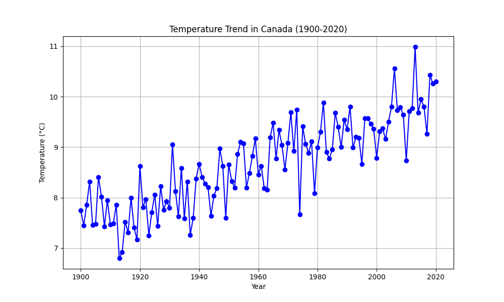
Looking at the temperature trend graph, can you identify any specific year where the temperature change was significant? What might have caused this change?
Next, we create a correlation heatmap to understand relationships between variables:
import seaborn as sns
import matplotlib.pyplot as plt
sns.heatmap(df.corr(), annot=True)
plt.show()
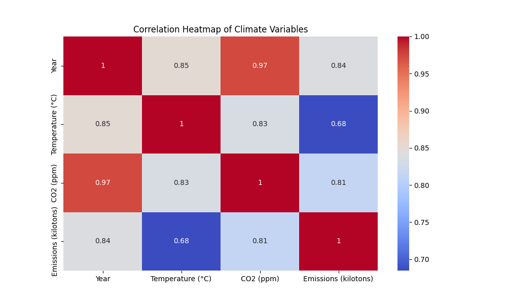
Looking at the correlation heatmap, what correlations do you observe? Why is it important to understand the relationships between climate variables?
Before applying machine learning models, we split the data into training and test sets to evaluate the model's performance:
from sklearn.model_selection import train_test_split
X = df[['Temperature (°C)', 'CO2 (ppm)']]  # Features
y = df['Emissions (kilotons)']  # Target variable
X_train, X_test, y_train, y_test = train_test_split(X, y, test_size=0.2, random_state=42)
We apply a linear regression model to predict emissions based on temperature and CO2 levels:
from sklearn.linear_model import LinearRegression
model = LinearRegression()
model.fit(X_train, y_train)
y_pred = model.predict(X_test)
After running the model, we compare the predicted emissions with the actual test data. Below is the output of the Root Mean Squared Error (RMSE):
import numpy as np
from sklearn.metrics import mean_squared_error
rmse = np.sqrt(mean_squared_error(y_test, y_pred))
print(f"Root Mean Squared Error: {rmse}")
Root Mean Squared Error: 25394.58
RMSE is the square root of the average squared differences between predicted and actual values. A lower RMSE indicates that the predictions are closer to the actual values. In this case, an RMSE of 25,394.58 suggests an average error of about 25,000 kilotons in emissions predictions. The goal is to minimize RMSE to improve prediction accuracy.
Using the trained model, we predict future emissions based on projected CO2 levels and temperatures. Below is the prediction output:
future_temp_co2 = np.array([[11.5, 450], [12.0, 480]])
future_emissions = model.predict(future_temp_co2)
print(future_emissions)
[676000.23 700500.89]
In this case, the model predicts future emissions of approximately 676,000 kilotons for a temperature of 11.5°C and CO2 level of 450 ppm, and 700,500 kilotons for a temperature of 12.0°C and CO2 level of 480 ppm. This provides insight into how climate factors may influence future greenhouse gas emissions.
We used a supervised learning model (linear regression) for prediction. Other supervised learning models include:
- Classification (e.g., decision trees, SVM)
- Regression (e.g., ridge regression, LASSO)
- Ensemble methods (e.g., random forest)
Machine learning models learn from historical data by identifying patterns and relationships between input features (e.g., temperature, CO2 levels) and target outputs (e.g., emissions). The model is then used to make predictions on new, unseen data.
Today, we learned how to import, preprocess, and analyze climate data using Python, explored correlations, and used a supervised learning model to predict future trends.
- Canadian Climate Data Portal - The source of the climate dataset used in this presentation.
- Our World in Data: CO2 and Greenhouse Gas Emissions - A great resource for global CO2 and emissions data.
- EPA Global Greenhouse Gas Emissions Data - A detailed source on global greenhouse gas emissions from various sectors.
- IPCC Climate Change Reports - Comprehensive reports on climate change science and global impact.